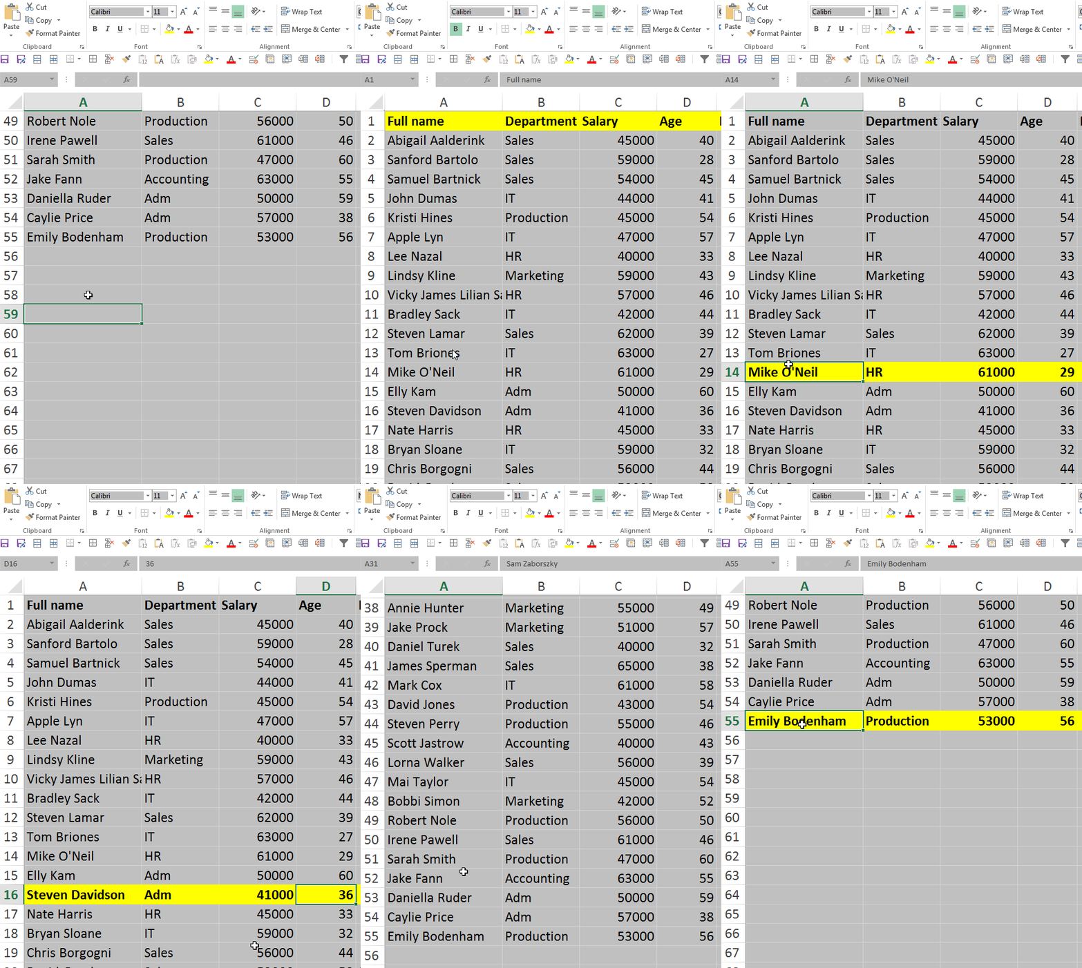
EXCEL – Highlight Active Row/Column when Cell is Selected (VBA)

IMPORTANT NOTE: THE EXCEL FILE MUST BE SAVED AS A MACRO-ENABLED DOCUMENT (XLSM).

Think that you have loads of data with 6000 rows (or more, or less, it doesn’t matter) and you need to watch them daily for details. You might miss things after concentrating on it for too much, clicking on a row and reading the data from the row above or below. Want to avoid that without highlighting each row using the fill command, then removing highlight? You might possibly ruin highlight that you already have in your sheet.

Note: selecting multiple rows or columns won’t highlight all of them, just the one that began the selection. I might post in the future a tutorial for selecting and highlighting multiple rows, so stay tuned.

The solution below doesn’t mess with previous cell fill, font color or whatever formatting you have in place.

The solution below also allows you to do it multiple times in the same sheet for multiple ranges, with different highlighting options. You can do part A multiple times for multiple ranges in the same sheet. Part B only has to be done once for a sheet (multiple times if multiple sheets, once for each).

A. Conditional formatting – depending on the formula you use, you either highlight only the row or both the row and the column (see point 4)

B. VBA code – this part is for moving the highlight when you click your mouse on a different cell, and it is why you will have to save your document as an Excel Macro-Enabled Workbook (XLSM)

A. Conditional formatting

1. Select the desired range of cells where you want the code to work – it can be for example A1:E55 or A5:AD10000 or whatever

You can select cells with data or blank cells, it doesn’t matter.

2. On the HOME tab click on Conditional Formatting and select New Rule

3. Select “Use a formula to determine which cells to format”

4. In the field enter either of the two formulas below:

a) If you just want to highlight the row (like in the picture above):  =OR(CELL("row")=CELL("row";A1))

Replace A1 in the formula above with the first cell of your range – for example for A5:AD10000 you have to replace A1 above with A5

b) If you want to highlight both the row and the column where your cell is: =OR(CELL("col")=COLUMN();CELL("row")=ROW())

5. Click the Format button and select the desired formatting – I usually use bold font and yellow fill, but you can use white font and red fill etc.

6. When ready click OK and then OK again

B. VBA code

1. Right click on the sheet name and select View Code to open the Microsoft Visual Basic for Applications window

2. In the window that opens paste the following lines of code:

Option Explicit
Private Sub Worksheet_SelectionChange(ByVal Target As Range)
Target.Calculate
End Sub

This it how it should look like (don’t worry if the left “tree” part is not showing – you can see it by going to View – Project Explorer):

3. Close the Microsoft VBA window (not the Excel file)

4. Save the file as an Excel Macro-Enabled Workbook (.XLSM)

THAT’S IT!

 

Similar tutorials:

Highlight the active Row with an underlining shape (line, rectangle etc.)

TBA – Highlight the active Row and Column left and above of the selected cell

TBA – Highlight the active Row and Column with colored borders

TBA – Highlight multiple Rows and Columns at once